Errata for "Student Solutions Manual for Nonlinear Dynamics and Chaos, Third Edition" by Mitchal Dichter

2.4.7
Please see the errata for the second edition below. This correction is present in both editions as it was not found until after the third edition was released.
Errata for "Student Solutions Manual for Nonlinear Dynamics and Chaos, Second Edition" by Mitchal Dichter

2.4.7
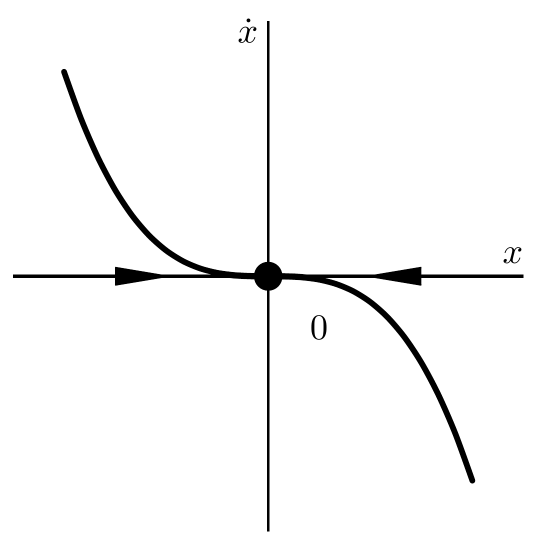
The plot of $\dot{x}$ mistakenly used $x^{3}$ instead of $-x^{3}$ which changes the stability from unstable to stable. The solution was also confusingly written for the $a \leq 0$ case. A correct and clearer version is below.
\begin{equation*}
\dot{x} = ax-x^{3} = x(\sqrt{a}-x)(\sqrt{a}+x)
\end{equation*}
\begin{equation*}\frac{\text{d}\dot{x}}{\text{d}x} = a-3x^{2}
\end{equation*}
There are three real fixed points $x= 0, \pm\sqrt{a}$ for $0 < a$ and one fixed point for $a \leq 0$ since the other two roots $x= \pm\sqrt{a}$ are either imaginary or coincide at zero.
\begin{align*}
&\frac{\text{d}\dot{x}}{\text{d}x}(-\sqrt{a}) = -2a \Rightarrow
\left\{
\begin{array}{lr}
\text{see 0 root in this case} & : a = 0 \\
\text{stable} & : 0 < a
\end{array}
\right. \\
\\
&\frac{\text{d}\dot{x}}{\text{d}x}(0) = a \Rightarrow
\left\{
\begin{array}{lr}
\text{inconclusive, but graph implies stable} & : a = 0 \\
\text{unstable} & : 0 < a
\end{array}
\right. \\
\\
&\frac{\text{d}\dot{x}}{\text{d}x}(\sqrt{a}) = -2a \Rightarrow\left\{
\begin{array}{lr}
\text{see 0 root in this case} & : a = 0 \\
\text{stable} & : 0 < a
\end{array}
\right.
\end{align*}
3.2.1
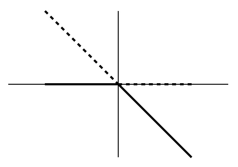
The bifurcation diagram is incorrect. The correct bifurcation diagram is
3.2.5
The last equation $= c_{1}-c_{2}x_{2}$ should be $= c_{1}x-c_{2}x^{2}$.
3.3.1 b)
The "p" in the bottom of the fraction on the last line should not be there.
3.3.1 d)
Extra parenthesis in $|GN-k| \ll |Gn+f|$ in the last paragraph.
3.5.7 c)
The $\kappa = rt$ on the last line should be $\displaystyle \kappa = \frac{N_{0}}{K}$.
3.6.5 a)
The second equation with $\displaystyle = -kx \left( 1 - \frac{L_{0}}{\sqrt{x^{2}+a^{2}}} \right)$ should be $\displaystyle = kx \left( 1 - \frac{L_{0}}{\sqrt{x^{2}+a^{2}}} \right)$ with no minus sign.
3.6.5 e) and 3.6.5 f)
The fraction $\displaystyle \frac{u^{4}+3u^{2}}{2(1-u^{2})}$ near the end of parts e) and f) should be $\displaystyle \frac{u^{4} + 6u^{2}}{2(2-u^{2})}$.
4.5.1 b)
The third equation $\displaystyle -\frac{\pi}{2}A \leq \frac{\Omega - \omega}{A} \leq \frac{\pi}{2}A$ should be $\displaystyle -\frac{\pi}{2}A \leq \Omega - \omega \leq \frac{\pi}{2}A$.
4.5.1 d)
The bounds of integration were plugged in backwards in the last two equations. The second to last equation should be $\displaystyle = \frac{2}{A}\left(\ln\left(\Omega-\omega-A\frac{-\pi}{2}\right)-\ln\left(\Omega-\omega-A\frac{\pi}{2}\right)\right)$ and the last equation should be $\displaystyle = \frac{2}{A}\left(\ln\left(\Omega-\omega+A\frac{\pi}{2}\right)-\ln\left(\Omega-\omega-A\frac{\pi}{2}\right)\right)$.
5.1.11 a)
The last line $\displaystyle \delta < \big|x_{0}\big| \Rightarrow \big|\big|\big(x(t),y(t)\big)\big|\big| < 2\big|x_{0}\big| = \epsilon$ should be $\displaystyle \big|\big|(x_{0},y_{0}\big)\big|\big| < \delta \Rightarrow \big|\big|\big(x(t),y(t)\big)\big|\big| < 2\delta = \epsilon$.
6.3.9 c)
Due to a very interesting and subtle assumption in the exercise, there is something wrong with the reasoning in part (c). Finding $u(t)$ this way assumes that $x(t)$ and $y(t)$ are defined for all time $t$, which isn't true. Turns out the $y^{3}$ terms in the $\dot{x}$ and $\dot{y}$ equations cause $x(t)$ and $y(t)$ to go to infinity in finite time for most initial conditions. (Solve $\dot{y}=y^{3}$ and you'll see why solutions blow up in finite time.) This is also apparent from the phase portrait in part (e).
So in fact what happens is the trajectories that escape to infinity asymptote to lines of the form $y = x + c$, since $y(t) - x(t)$ will decay exponentially to some constant $c$ as $t$ approaches the finite blow up time.
6.4.11 b)
The eigenvalues for matrix $\displaystyle A_{(0,0,z)}$ should be changed from $\displaystyle \lambda_{1} = 0 \quad \lambda_{2} = 0 \quad \lambda_{3} = rz$ to $\displaystyle \lambda_{1} = rz \quad \lambda_{2} = rz \quad \lambda_{3} = 0$.
6.5.7 c)
\begin{align}
&A = \begin{pmatrix}
0 & 1 \\
2\epsilon u - 1 & 0
\end{pmatrix} \\
&A_{\left(\frac{1+\sqrt{1-4\alpha\epsilon}}{2\epsilon},0\right)} = \begin{pmatrix}
0 & 1 \\
\sqrt{1-4\alpha\epsilon} & 0
\end{pmatrix} \\
&\Delta = -\sqrt{1-4\alpha\epsilon} \quad \tau = 0 \Rightarrow \text{Saddle point} \\
&A_{\left(\frac{1-\sqrt{1-4\alpha\epsilon}}{2\epsilon},0\right)} = \begin{pmatrix}
0 & 1 \\
-\sqrt{1-4\alpha\epsilon} & 0
\end{pmatrix} \\
&\Delta = \sqrt{1-4\alpha\epsilon} \quad \tau = 0 \Rightarrow \text{Linear Center}
\end{align}
This is also a nonlinear center by Theorem 6.5.1 with the only difficult condition to check is that the fixed point is a local minimum of a conserved quantity.
\begin{align}
&E = \frac{1}{2}\dot{x}^{2} + \int -(\alpha+\epsilon x^{2} - x) \text{ d}x = \frac{1}{2}\dot{x}^{2} - \alpha x - \frac{\epsilon}{3}x^{3} + \frac{1}{2}x^{2} \\
&\nabla E = \langle \alpha+\epsilon x^{2} - x , \dot{x} \rangle \\
&\nabla E\left(\frac{1-\sqrt{1-4\alpha\epsilon}}{2\epsilon},0\right) = (0,0)
\end{align}
\begin{align}
\begin{vmatrix}
E_{xx} & E_{x\dot{x}} \\
E_{\dot{x}x} & E_{\dot{x}\dot{x}}
\end{vmatrix} &= \begin{vmatrix}
-2\epsilon x+1 & \dot{x}-\alpha-\epsilon x^{2}+x \\
\dot{x}-\alpha-\epsilon x^{2}+x & 1
\end{vmatrix} \\
&= -2\epsilon x+1 - (\dot{x}-\alpha-\epsilon x^{2}+x)^{2}
\end{align}
$\nabla E = (0,0)$ at the fixed fixed point. Both $E_{xx}, E_{\dot{x}\dot{x}} > 0$ at the fixed point for sufficiently small $\epsilon$, as well as the evaulation of the Jocobian at the fixed point,
\begin{equation}
\begin{vmatrix}
E_{xx} & E_{x\dot{x}} \\
E_{\dot{x}x} & E_{\dot{x}\dot{x}}
\end{vmatrix}_{\left(\frac{1-\sqrt{1-4\alpha\epsilon}}{2\epsilon},0\right)} = \sqrt{1-4\alpha\epsilon} > 0 \Rightarrow \left(\frac{1-\sqrt{1-4\alpha\epsilon}}{2\epsilon},0\right) \text{is a local minimum.}
\end{equation}
7.2.7 a)
The partial derivatives should be reversed to $\displaystyle \frac{\partial}{\partial y}\big(y+2xy\big) = 1+2x = \frac{\partial}{\partial x}\big(x+x^{2}-y^{2}\big)$.
7.3.1 e)
The bottom half should be
$\displaystyle \frac{1}{1+\sin^{2}(2\theta)} = \frac{-1}{4\cos(\theta)\sin^{3}(\theta)} \Rightarrow 4\cos(\theta)\sin^{3}(\theta) = -1-\sin^{2}(2\theta)$
Determining the solutions of this equation is difficult analytically, but graphically it's pretty clear that there are no real solutions to the equation.
7.3.7 a)
The last line $= 2ab\sin(2\theta)-1$ should be $= ab\sin(2\theta)-1$.
7.3.9 a)
The last line $\displaystyle r_{1} = \frac{1}{5}\sin(t)+\frac{2}{5}\cos(\theta) + Ce^{-2t}$ should be $\displaystyle r_{1} = \frac{1}{5}\sin(\theta)+\frac{2}{5}\cos(\theta) + Ce^{-2\theta}$.
7.5.3
There was an erroneous $+z$ to the left of the second equals.
\begin{equation}
0 = \ddot{z}+k\big((z+1)^{2}-4\big)\dot{z} =\frac{\text{d}}{\text{d}t} \left(\dot{z}+k\left(\frac{1}{3}(z+1)^{3}-4z\right)\right)
\end{equation}
The limit cycle was assumed to be symmetric and is not, so both branches must be computed.
\begin{equation}
T \approx \int_{t_{A}}^{t_{B}} \text{ d}t + \int_{t_{C}}^{t_{D}} \text{ d}t = -k\left( \int_{3}^{1} \frac{(z+1)^{2}-4}{z} \text{ d}z + \int_{-5}^{-3} \frac{(z+1)^{2}-4}{z} \text{ d}z \right) = k\big(12-3\ln(5)\big)
\end{equation}
The $\displaystyle 2k \ln\big(8 − \ln(27)\big)$ should be $\displaystyle 2k \big(8 − \ln(27)\big)$ without the first $\displaystyle \ln$.
7.6.3 b)
The initial conditions were applied incorrectly. The correct equations are,
\begin{align}
&\ddot{x}_{0}+x_{0} = 0 \Rightarrow x_{0} = \cos(t) \\
&\ddot{x}_{2}+x_{2} = 0 \Rightarrow x_{2} = 0 \\
&\ddot{x}_{1}+x_{1} - 1 = 0 \Rightarrow x_{1} = 1-\cos(t)
\end{align}
and
\begin{align}
x(t,\epsilon) &= x_{0}(t,\epsilon) + \epsilon x_{1}(t,\epsilon) + \epsilon^{2}x_{2}(t,\epsilon) + O\big(\epsilon^{3}\big) \\
&\approx \cos(t) + \epsilon\big(1-\cos(t)\big) = \epsilon + (1-\epsilon)\cos(t)
\end{align}
7.6.15 a)
There were many errors. Here is the corrected segment.
\begin{align}
\frac{\text{d}r}{\text{d}T} &= \langle h\sin(\theta) \rangle = \frac{1}{2\pi} \int_{0}^{2\pi} h\big(r\cos(\theta),-r\sin(\theta)\big)\sin(\theta) \text{ d}\theta \\
&= \frac{1}{2\pi} \int_{0}^{2\pi} -r^{3}\cos^{3}(\theta)\sin(\theta) \text{ d}\theta = 0 \Rightarrow r(T) = r_{0} \\
r\frac{\text{d}\phi}{\text{d}T} &= \langle h\cos(\theta) \rangle = \frac{1}{2\pi} \int_{0}^{2\pi} h\big(r\cos(\theta),-r\sin(\theta)\big)\cos(\theta) \text{ d}\theta \\
&= \frac{1}{2\pi} \int_{0}^{2\pi} -r^{3}\cos^{4}(\theta) \text{ d}\theta = -\frac{3}{8}r^{3} \\
\frac{\text{d}\phi}{\text{d}T} &= -\frac{3}{8}r^{2}
\end{align}
\begin{equation}
r(0) = \sqrt{x(0)^{2}+\dot{x}(0)^{2}} = a \qquad r(T) = a
\end{equation}
\begin{equation}
\omega = 1 + \epsilon\phi' = 1 - \epsilon \frac{3}{8}r_{0}^{2} + O\big(\epsilon^{2}\big) \approx 1 - \frac{1}{16}a^{2}
\end{equation}
8.1.15 c)
One of the matrices at the bottom of part (c) was transposed. There was also an unnecessary matrix at the bottom. Here is the corrected version.
\begin{equation}
A = \begin{pmatrix}
\frac{\text{d}}{\text{d}n_{A}}\dot{n}_{A} & \frac{\text{d}}{\text{d}n_{B}}\dot{n}_{A} \\
\frac{\text{d}}{\text{d}n_{A}}\dot{n}_{B} & \frac{\text{d}}{\text{d}n_{B}}\dot{n}_{B}
\end{pmatrix} = \begin{pmatrix}
-2n_{A}-2n_{B}-2p+1 & -2n_{A}-2p \\
-2n_{B} & -2n_{A}-2n_{B}-p+1
\end{pmatrix}
\end{equation}
\begin{equation}
A_{(1-p,0)} = \begin{pmatrix}
-1 & -1 \\
0 & p-1
\end{pmatrix} \qquad \lambda_{1} = -1 \quad \lambda_{2} = p-1
\end{equation}
8.6.7 c)
The simplification for the winding number had a missing $\sqrt{3}$ in the second fraction.
\begin{equation}
\frac{\omega_{r}}{\omega_{\theta}} = \frac{\sqrt{3}\omega_{\theta}}{\omega_{\theta}} = \sqrt{3}
\end{equation}
8.7.3 c)
The explanation for the limits as $T \rightarrow 0$ and $T \rightarrow \infty$ were poorly written, wrong, and ambiguous. Here is the rewritten part (c).
Using the equation derived from part (a)
\begin{align}
&\lim_{T\rightarrow 0} x(T) = \lim_{T\rightarrow 0} e^{-T}x_{0} - A\big(1-e^{-\frac{T}{2}}\big)^{2} = x_{0} - A\big(1-1\big)^{2} = x_{0} \\
&\lim_{T\rightarrow \infty} x(T) = \lim_{T\rightarrow \infty} e^{-T}x_{0} - A\big(1-e^{-\frac{T}{2}}\big)^{2} = (0)x_{0} - A\big(1-0\big)^{2} = -A
\end{align}
The first result is quite plausible. As the period goes to zero then the forcing function $F(t)$ has almost no time to do anything and $x(t)$ has no time to move anywhere within one $T$-length period. If $x(0) = x_{0}$ then $x(T) \approx x(0) = x_{0}$ as $T \rightarrow 0$. The solution has virtually no time to change.
The second result is intuitive by letting $T$ be large, which in this context means $T \gg 1$. Why is that the correct condition? Because for the equation in question, the rate constant for exponential decay, and hence its inverse, the time scale, are both equal to 1. We can see that by looking at the coefficient of $x$ in the equation
\begin{equation}
\dot{x} + x = \pm A.
\end{equation}
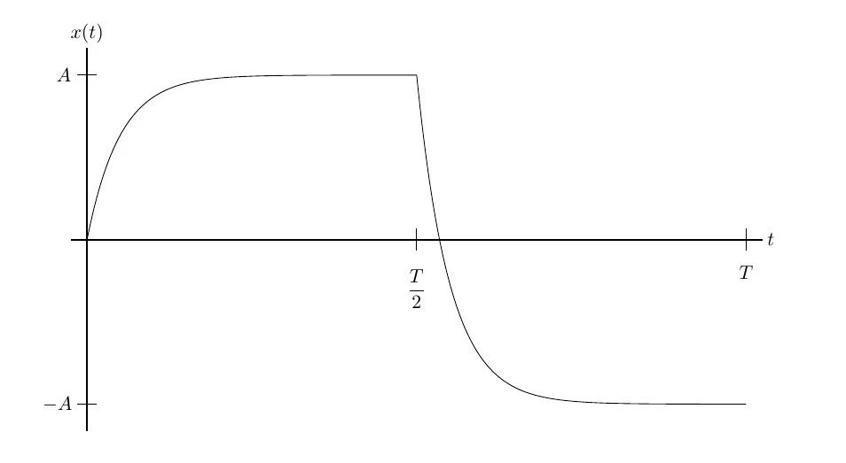
So, how does $x(t)$ behave for large $T$? Well, at first the value of $x(t)$ relaxes exponentially fast, on a time scale of 1, to a value of $x \approx A$. It stays there as the time dawdles its way up to $t = \frac{T}{2}$. Then, in the second half of the forcing cycle, we switch the value of $F(t)$ to $-A$. By the same reasoning as before, $x$ then moves exponentially fast to $x \approx -A$. It essentially stays at $x = -A$ until the end of the cycle at $t =T$.
What makes this reasoning valid (asymptotically, for $T \gg 1$) is that the relaxation to the equilibrium happens on a much faster time scale than the switching of $F$.
This all becomes very clear visually by plotting $x(t)$ for a moderately large forcing period. For instance, $T = 20$, $A = 3$, and $x(0)=0$.
8.7.9 a)
The expression for $r(t)$ is incorrect. The $2\pi$'s should be $t$'s.
\begin{equation}
r(t) = \frac{e^{t}r_{0}}{(e^{t}-1)r_{0}+1}
\end{equation}
9.5.5 a)
The was a mistake in the derivative of the $z$ term. A 1 should have turned into a 0 which propagated through the problem. Here are the corrected pieces.
\begin{equation}
\dot{z} = \frac{1}{\sigma\epsilon^{3}}\frac{\text{d}Z}{\text{d}\tau} = xy-bz = \frac{X}{\epsilon}\frac{Y}{\epsilon^{2}\sigma}-b\frac{1}{\epsilon^{2}}\left(\frac{Z}{\sigma}+1\right)
\end{equation}
\begin{equation}
\frac{1}{\sigma\epsilon^{3}}\frac{\text{d}Z}{\text{d}\tau} = \frac{X}{\epsilon}\frac{Y}{\epsilon^{2}\sigma}-b\frac{1}{\epsilon^{2}}\left(\frac{Z}{\sigma}+1\right) \Rightarrow \frac{\text{d}Z}{\text{d}\tau} = XY-b\epsilon\left(Z+\sigma\right) \qquad \lim_{\epsilon \rightarrow 0} \frac{\text{d}Z}{\text{d}\tau} = XY
\end{equation}
10.1.9
\begin{equation}
f'(x) = \frac{2(1+x)-2x(1)}{(1+x)^{2}} = \frac{2}{(1+x)^{2}}
\end{equation}
10.1.11 d)
\begin{align}
|x_{1}| &= |3x_{0}-x_{0}^{3}| = |x_{0}||3-x_{0}^{2}| = |x_{0}||3-(2 + \epsilon)^{2}| \\
&= |x_{0}||3-(4 + 4\epsilon + \epsilon^{2})| = |x_{0}||-1 - 4\epsilon - \epsilon^{2})| \\
&= |x_{0}|(1 + 4\epsilon + \epsilon^{2})
\end{align}
10.2.1 a)
\begin{equation}
x_{n+1} - x_{n} = -r\epsilon(1 + \epsilon) - (1 + \epsilon) = -(r \epsilon+1)(1 + \epsilon) < -r \epsilon
\end{equation}
So the sequence decreases by at least $r \epsilon$ every iteration.
10.3.3
I incorrectly wrote the square roots as $\pm\sqrt{1-r}$ when it should be $\pm\sqrt{r-1}$ which changed several parts of the problem.
\begin{equation}
x = 0,\pm\sqrt{r-1}
\end{equation}
So there are three fixed points for $1< r$ and one fixed point for $r \le 1$.
\begin{equation}
f'(\pm\sqrt{r-1}) = \frac{2}{r} - 1 \qquad r < 1 \Rightarrow x^{*} = 0 \text{ is stable}
\end{equation}
\begin{equation}
1 < r \Rightarrow x^{*} = 0 \text{ is unstable, and } x^{*} = \pm\sqrt{r-1} \text{ are stable}
\end{equation}
10.3.11 a)
\begin{equation}
-1 < -(1+r) < 1 \Rightarrow -2 < r < 0
\end{equation}
\begin{equation}
-2 < r < 0 \Rightarrow \text{Stable} \qquad r < -2 \text{ or } 0 < r \Rightarrow \text{Unstable}
\end{equation}
10.3.11 b)
\begin{align}
&r < 0 \Rightarrow f'(0) = -(1+r) > -1 \Rightarrow \text{Stable} \\
&0 < r \Rightarrow f'(0) = -(1+r) < -1 \Rightarrow \text{Unstable}
\end{align}
11.2.1
The step
\begin{equation}
= 1-\frac{1}{3}\sum_{n=0}^{\infty}\left(\frac{2}{3}\right)^{n}
\end{equation}
is missing the $n$ in the exponent.
11.3.1 b)
The step
\begin{equation}
= 1-\frac{1}{2}\sum_{n=0}^{\infty}\left(\frac{1}{2}\right)^{n}
\end{equation}
is missing the $n$ in the exponent.
11.4.1
The diagrams of the boxes overlaid on iterations of the Koch snowflake should be overlaid on the complete Koch snowflake. The box counting is computed for the fractal, not each iteration of constructing the fractal.
11.4.9
Missing power of $n$ added to $N(\epsilon) = (p^{2}-m^{2})^{n}$.
12.2.11
Change $x_{n}$ to $x_{0}$ in $x_{1} = y_{0}+1-ax_{0}^{2}$.